蒙特卡洛就是— 用大量随机试验,去逼近一个本来很难算的结果 ;它不是“高深算法”,而是一种思想:“既然精确算不出来,那就随机抽样,统计平均。”
(知识不管看不看,记得在文末领小星球红包封面)
最经典的例子:算圆周率 π
有一个正方形,里面画一个内切圆,如果往随机往正方形里撒 100 万个点,然后统计有多少点落在圆里
那么:
蒙特卡洛就是— 用大量随机试验,去逼近一个本来很难算的结果 ;它不是“高深算法”,而是一种思想:“既然精确算不出来,那就随机抽样,统计平均。”
(知识不管看不看,记得在文末领小星球红包封面)
有一个正方形,里面画一个内切圆,如果往随机往正方形里撒 100 万个点,然后统计有多少点落在圆里
那么:
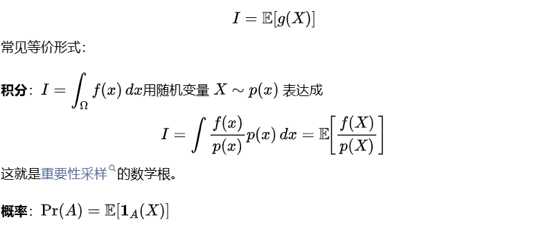
当遇到:积分算不出来,系统误差难以解析,多变量耦合太复杂,概率分布太复杂
蒙特卡洛说:
别推公式了,直接模拟。
因为一个很朴素的事实:
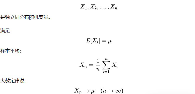
如果随机样本足够多,平均值就会接近真实值。
这就是大数定律。
简单说:
10 次试验 → 很不准
1000 次 → 还可以
100 万次 → 非常接近
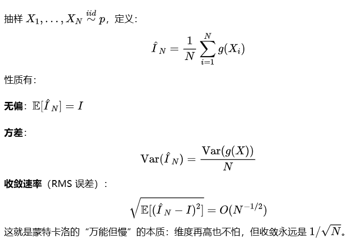
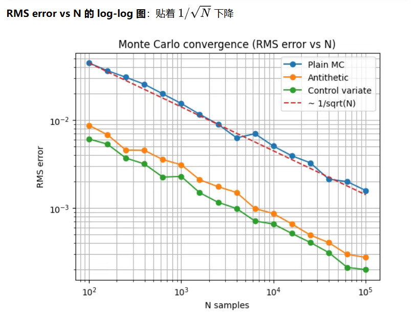
误差大约按:

所以样本翻 4 倍,误差减半。

意思是:偏离真实值的概率 → 0,这是“概率意义下收敛”。
关键是每个随机变量有波动,但独立波动会互相抵消;假设每个变量方差为 ,那么平均值的方差:
波动幅度随 1/√n 下降
样本越多,平均值越稳定。
蒙特卡洛本质就是:
比如我们测电压:真实值 = 10.000000 V,但是每次测量带有噪声,然后连续测 N 次,取平均;那么测量误差标准差会变成:

这就是为什么:DMM 用积分,ADC 用平均,低频噪声用长时间统计的一点点数学解释。
很多人会混淆。(我也之前没有完全明白)
| 名称 | 讲什么 |
|---|---|
| 大数定律 | 平均值会收敛 |
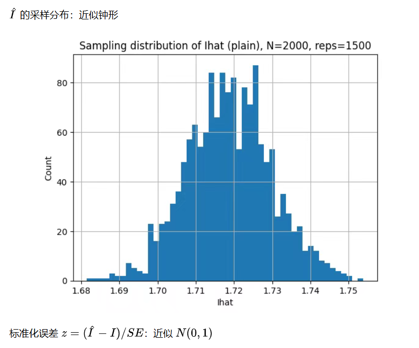
| 中心极限定理 | 平均值的分布会变成正态 |
大数定理它告诉我们一个哲学事实:
不确定性可以通过重复消除。
这几乎是统计学和工程的根基。
比如在金融领域:算复杂期权定价,算极端风险概率(公式算不了,只能随机模拟未来市场);物理领域可以计算粒子碰撞模拟,也可以热噪声统计。
在IC 里面可以做器件误差分析,比如:电阻 ±1%,运放偏置 ±50µV,参考源 ±10ppm,书面的很难推一个复杂误差传播公式;但可以:随机生成一组参数,算一次输出,重复 10 万次,看输出分布,这就是工程里的蒙特卡洛。
另外蒙特卡洛不是乱随机,它是:先建模型,再随机输入,最后统计输出;例如:输出 = f(电阻, 温度, 噪声),把电阻 ~ 正态分布,温度 ~ 均匀分布,噪声 ~ 高斯白噪声,代进去随机跑 10 万次。最后得到:输出的均值,输出的标准差, 输出的概率分布;可以叫做概率建模 + 随机求解。(缺点是收敛慢(1/√N)需要大量计算。)
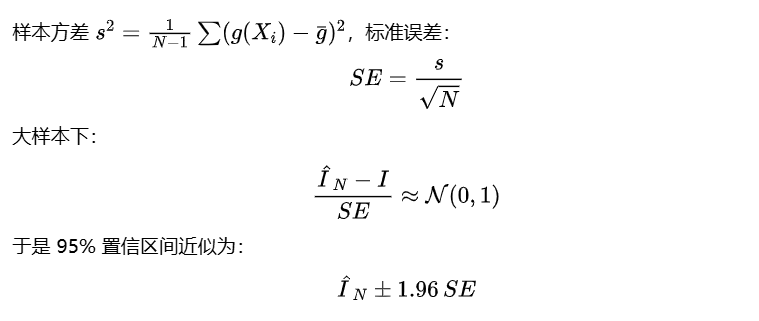
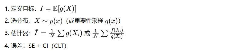
置信区间:把“不确定度”量化出来
用一个标准例子演示:
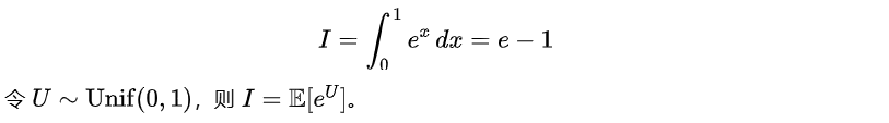
Target I = ∫_0^1 exp(x) dx = e - 1 = 1.718281828459045
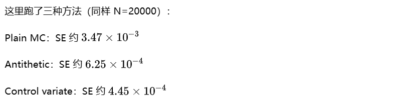
Plain : Ihat=1.72215757, SE=3.466e-03, 95% CI=(np.float64(1.7153641635016394), np.float64(1.7289509773653648))
Antithetic : Ihat=1.71772080, SE=6.245e-04, 95% CI=(np.float64(1.7164966886828101), np.float64(1.7189449125866085))
ControlVar : Ihat=1.71855180, SE=4.446e-04, 95% CI=(np.float64(1.7176804373321641), np.float64(1.7194231571928984)), b≈1.6884
蒙特卡洛这篇文章不是空穴来风,是因为最近在研究传感器,建模了不少的东西,后面在做整体评估的时候就不免的使用蒙特卡洛,然后就萌生这个写作的想法。
import numpy as np
import matplotlib.pyplot as plt
# =========================
# Monte Carlo: mathematical modeling + simulation demo (fast version)
# =========================
# Target: I = ∫_0^1 exp(x) dx = e - 1 = E[exp(U)], U ~ Unif(0,1)
# Show:
# - Estimator + 95% CI
# - Convergence ~ 1/sqrt(N)
# - Variance reduction: antithetic + control variate
# - CLT intuition via standardized errors
# =========================
TRUE_I = np.e - 1.0
def mc_plain(N, rng):
u = rng.random(N)
y = np.exp(u)
Ihat = y.mean()
se = y.std(ddof=1) / np.sqrt(N)
return Ihat, se
def mc_antithetic(N_total, rng):
# Use N_total samples by pairing => N_pairs = N_total/2
N_pairs = N_total // 2
u = rng.random(N_pairs)
z = 0.5 * (np.exp(u) + np.exp(1.0 - u))
Ihat = z.mean()
se = z.std(ddof=1) / np.sqrt(N_pairs)
return Ihat, se
def mc_control(N, rng):
u = rng.random(N)
x = np.exp(u)
c = u
c0 = 0.5
cov = np.cov(x, c, ddof=1)[0, 1]
varc = np.var(c, ddof=1)
b = cov / varc
z = x - b * (c - c0)
Ihat = z.mean()
se = z.std(ddof=1) / np.sqrt(N)
return Ihat, se, b
def ci95(Ihat, se):
return (Ihat - 1.96*se, Ihat + 1.96*se)
# ---- Single run summary
rng = np.random.default_rng(0)
N = 20000
I1, se1 = mc_plain(N, rng)
I2, se2 = mc_antithetic(N, rng)
I3, se3, b3 = mc_control(N, rng)
print("Target I = ∫_0^1 exp(x) dx = e - 1 =", TRUE_I)
print(f"Plain : Ihat={I1:.8f}, SE={se1:.3e}, 95% CI={ci95(I1,se1)}")
print(f"Antithetic : Ihat={I2:.8f}, SE={se2:.3e}, 95% CI={ci95(I2,se2)}")
print(f"ControlVar : Ihat={I3:.8f}, SE={se3:.3e}, 95% CI={ci95(I3,se3)}, b≈{b3:.4f}")
# ---- Convergence study (reduced)
Ns = np.unique(np.logspace(2, 5, 16).astype(int)) # 1e2..1e5, 16 points
n_rep = 60 # repetitions per N
def rms_error(method, N, seed_base=123):
errs = np.empty(n_rep)
for k in range(n_rep):
rg = np.random.default_rng(seed_base + 10000*k + N)
if method == "plain":
Ihat, _ = mc_plain(N, rg)
elif method == "antithetic":
Ihat, _ = mc_antithetic(N, rg)
elif method == "control":
Ihat, _, _ = mc_control(N, rg)
else:
raise ValueError
errs[k] = Ihat - TRUE_I
return np.sqrt(np.mean(errs**2))
rms_plain = np.array([rms_error("plain", int(n)) for n in Ns])
rms_anti = np.array([rms_error("antithetic", int(n)) for n in Ns])
rms_ctrl = np.array([rms_error("control", int(n)) for n in Ns])
ref = rms_plain[0] * np.sqrt(Ns[0] / Ns)
plt.figure()
plt.loglog(Ns, rms_plain, marker="o", label="Plain MC")
plt.loglog(Ns, rms_anti, marker="o", label="Antithetic")
plt.loglog(Ns, rms_ctrl, marker="o", label="Control variate")
plt.loglog(Ns, ref, linestyle="--", label="~ 1/sqrt(N)")
plt.xlabel("N samples")
plt.ylabel("RMS error")
plt.title("Monte Carlo convergence (RMS error vs N)")
plt.grid(True, which="both")
plt.legend()
plt.show()
# ---- CLT intuition: standardized errors (reduced)
N_clt = 2000
reps = 1500
Ihats = np.empty(reps)
ses = np.empty(reps)
for k in range(reps):
rg = np.random.default_rng(7 + k)
Ihat, se = mc_plain(N_clt, rg)
Ihats[k] = Ihat
ses[k] = se
z = (Ihats - TRUE_I) / ses
plt.figure()
plt.hist(Ihats, bins=50)
plt.xlabel("Ihat")
plt.ylabel("Count")
plt.title(f"Sampling distribution of Ihat (plain), N={N_clt}, reps={reps}")
plt.grid(True)
plt.show()
plt.figure()
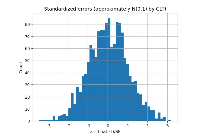
plt.hist(z, bins=50)
plt.xlabel("z = (Ihat - I)/SE")
plt.ylabel("Count")
plt.title("Standardized errors (approximately N(0,1) by CLT)")
plt.grid(True)
plt.show()